


In a previous post, we introduced our latest paper, which probes LLM internals through the lens of the Jacobian: the matrix that captures, to first order, what a single transformer layer does to the residual stream.
The residual stream is a wide vector that every layer reads from and writes back to: each block takes the current stream, computes, and adds its result. That running update is what makes a dynamical reading of transformer computation possible.
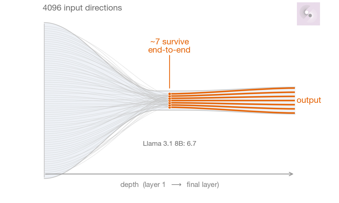
Llama 3.1 8B carries its computation in a residual stream 4,096 numbers wide—4,096 effective directions a thought could in principle move in. How many of those directions actually survive the trip from the model’s input to its output, 32 layers deep in Llama’s case? What hideous monsters must the signal battle along the way?
We found that the residual stream’s voyage is almost as epic as Odysseus’s: of the 4,096 directions it could start with, only about seven survive to the end. (Better odds than Odysseus’s men faced).
A model with eight billion parameters, operating a workspace four thousand dimensions wide, turns out to funnel almost everything it does through a channel you could count with your fingers. And it isn’t built that way. At the start of training the channel is wide; training squeezes it shut.
This post is about that squeeze—what it is, how we measured it, and a surgical experiment that tells us which part of the trained network is doing the actual squeezing. The answer turned out to be the same strange property we traced in our last post: the rotational, lopsided structure that makes a transformer’s layers non-normal.
First, a guardrail, because the number is easy to over-read.
“Seven dimensions survive” is not the claim that the model only knows seven things, or has seven features, or thinks seven tokens or thoughts. This is not the famous finding in psychology that human working memory taps out when dealing with more than seven items at a time (that paper, by George Miller, is worth a read nevertheless). The transformer is not persecuted by the integer seven, and plainly represents far more than seven concepts. The seven is a statement about sensitivity rather than content.
Take the trained model and nudge its input—perturb the residual stream by a tiny amount in some direction. Follow that nudge all the way through the layers to the output. Most directions you could push in get crushed to nothing along the way; the model is simply not sensitive to them by the time the signal reaches the end. Only about seven effective directions make it through with any strength intact. So the seven is the dimensionality of the channel through which an input perturbation can still move the output—the width of the model’s end-to-end responsiveness to its own input.
That’s a striking finding about a four-thousand-dimensional system. Through training, the network has evolved to ignore the overwhelming majority of the ways its own state could vary. Talk about being stuck in your ways.
How did we find this? Recall the Jacobian: the best linear stand-in for a layer. Each transformer layer takes the 4,096-dimensional residual stream in and hands a slightly modified one back, and its Jacobian is the 4,096 × 4,096 matrix that says, to first order, how a small change at the input becomes a small change at the output. One Jacobian per layer describes one step of the computation.
To follow a perturbation across the whole model, just multiply the per-layer Jacobians together. Compose them, layer 0 through the last layer, and you get a single matrix: the end-to-end linear map from a nudge at the input to the resulting wiggle at the output. This is the cumulative Jacobian, P. It’s the Jacobian of the entire stack, built by chaining the Jacobians of its parts.
Then we ask how concentrated that matrix is, using a quantity called effective rank. A matrix has a set of singular values—the gains along its principal directions. If a handful are large and the rest are near zero, the matrix is effectively low-dimensional: it really only acts along a few directions, no matter how big it nominally is. Effective rank turns that intuition into a single number. A 4,096 × 4,096 matrix with energy spread evenly across all its directions has an effective rank near 4,096; one whose energy collapses into a few directions has an effective rank in the single digits.
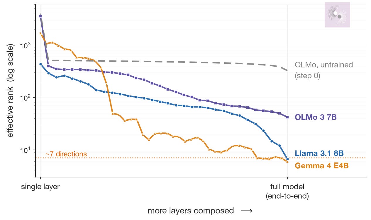
The cumulative Jacobian of Llama, composed end-to-end, has an effective rank of about 6.7. That’s the seven and it’s not just a quirk of Llama: we ran the same composition on two other models and on a third at multiple points in its training:
Llama 3.1 8B: ~7.
Gemma 4 E4B, a different architecture, 42 layers deep: ~6.
OLMo 3 7B, the model we have training checkpoints for: ~42 at the end of training.
Three production models, three architectures, the same shape of result: a four-thousand-dimensional workspace, an end-to-end channel orders of magnitude narrower.
We also have OLMo at step 0—i.e. random weights, before training, but same architecture and wiring as the trained version. At step 0 the effective rank of the full cumulative Jacobian is in the hundreds. The bottleneck isn’t in the architecture. Training installs it, progressively, squeezing a channel that started wide down toward a sliver. One can’t help but picture a camel squeezing through the eye of a needle.
Two suspects
So training builds a bottleneck. How? What is it about the trained matrices that funnels everything into seven directions?
There are two natural suspects, and they’re easy to confuse.
Suspect one: the eigenvalues. Every one of these Jacobians has a spectrum—a set of eigenvalues that say how much it amplifies or shrinks along its special directions. If a few of those are large and the rest are small, then composing many layers would amplify a few directions exponentially and starve the others. Repeated multiplication is unforgiving: a direction with gain slightly above 1, compounded over 32 layers, runs away; a direction with gain slightly below 1 vanishes. On this story, the bottleneck is just the arithmetic of the spectrum—the loud directions drown out the quiet ones.
Suspect two: the non-normal structure. A non-normal matrix is one whose input directions and output directions don’t line up—it takes things in along one set of axes and emits them along another, twisted set. Crucially, two matrices can have the exact same eigenvalues but completely different non-normal structure. The eigenvalues are only part of what a matrix is. There’s a second, off-the-books component—mathematicians would call it the strictly upper-triangular part in the right basis—that the eigenvalues don’t see at all. On this story, the bottleneck lives in that hidden component. It’s invisible to the spectrum, haunting it like a wraith.
What “non-normal” looks like. Both operators have the same eigenvalues (0.9 and 0.6, both below 1, so both ultimately contract). The normal operator on the left shrinks every input monotonically toward the origin. The non-normal operator on the right amplifies first—swinging vectors out past the unit circle (~2.3×) before they curl back and decay. Its input and output directions don’t line up. That gap is the non-normality, but the spectrum alone can’t see it.
The trouble is that you can’t tell the two apart by staring at the cumulative Jacobian. Both suspects produce the same low effective rank. To separate them you need to hold one fixed and vary the other—and for that, we needed a scalpel.
The Schur surgery
The scalpel is the Schur decomposition. Every square matrix has one, and the idea is this: Rotate the coordinate frame to just the correct set of perpendicular axes, and in those new coordinates the matrix becomes triangular: all of its action collapses onto and above the diagonal, with zeros below.
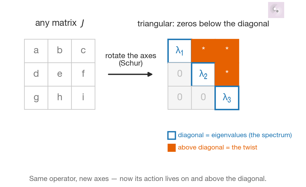
That triangular form is two pieces sitting in the same frame. The entries on the diagonal are the eigenvalues—the spectrum, suspect one. Everything strictly above the diagonal is the non-normal part—suspect two, the twisted feedforward coupling that a normal matrix simply doesn’t have. For a perfectly normal matrix that upper block is exactly zero; the further it is from zero, the more non-normal the matrix.
The catch is in those words “perpendicular axes.” Describing a matrix always means choosing a set of coordinate axes to measure it against—a ruler laid over space. Schur insists on a straight ruler: axes that are all the same length and meet at right angles, like ordinary graph paper. Mathematically this is a unitary change of basis; for complex eigenvalues, the clean version lives in complex coordinates.
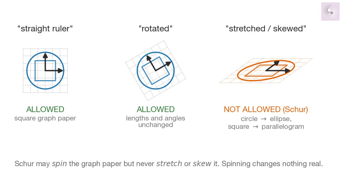
You’re allowed to spin that graph paper to any angle you like, but you can’t stretch it or skew it. Spinning is free because it changes nothing real—lengths stay lengths, right angles stay right angles, the matrix in the new frame is the same operator, just relabeled.
There’s a more familiar way to tidy up a matrix, and it’s worth seeing why we don’t use it. It’s called diagonalizing (rewriting the matrix so every entry off the diagonal is zero—the cleanest possible form, just a list of stretch factors along a set of special directions). Every matrix has a set of those special directions, its eigenvectors (the directions the matrix merely stretches or shrinks without rotating). When a matrix has a full set of eigenvectors, you can diagonalize it. Lay your ruler along the eigenvectors and the matrix looks perfectly diagonal—spotless, no twist anywhere.
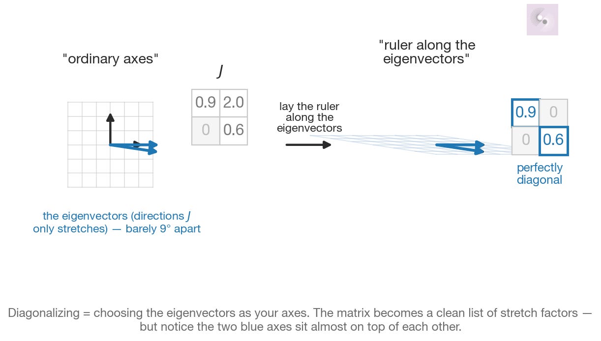
So why not always do that? Because for a non-normal matrix, the eigenvectors aren’t perpendicular to each other. They can sit at almost the same angle, nearly on top of one another. To lay your ruler along them, you have to bend the graph paper—skew the axes, squash one direction toward another. When you do that, the twist doesn’t disappear, it just stops looking like a twist. It gets folded into how crooked your ruler now is. Measure the model’s behavior on that skewed ruler and the dramatic amplification we care about reads as nothing special; convert back to honest, square-graph-paper lengths and it’s right back. The tidy diagonal was bought by lying about distances.
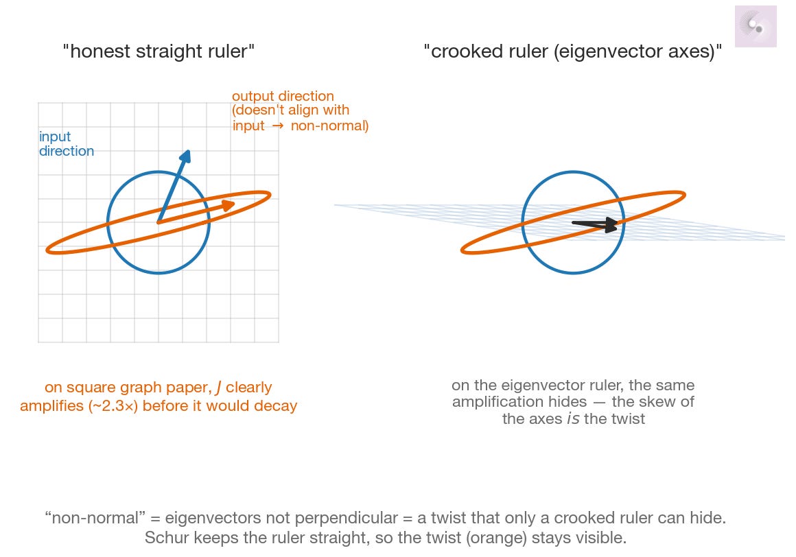
So “non-normal” and “eigenvectors that aren’t perpendicular” are two descriptions of the same fact. Schur refuses the crooked ruler: with the axes forced to stay perpendicular, the twist has nowhere to hide. It can’t be absorbed into a skewed frame, so it surfaces as the explicit block of numbers above the diagonal. One specific rotation, and the matrix falls cleanly into two parts—the eigenvalues on the diagonal (suspect one) and the twist above it (suspect two)—with nothing swept under the rug.
That split is exactly what we wanted, because it lets us operate on one while leaving the other untouched.
The two basis-change moves, side by side. Act 1 — diagonalizing makes the matrix tidy, but only by warping the ruler: the axes shear to ~8° apart and the twist gets absorbed into the skew. Act 2 — Schur’s move is a rigid rotation: the frame swivels without stretching, and the matrix splits cleanly into the eigenvalues on the diagonal (blue, the spectrum) and the twist above it (orange) — with nothing hidden.
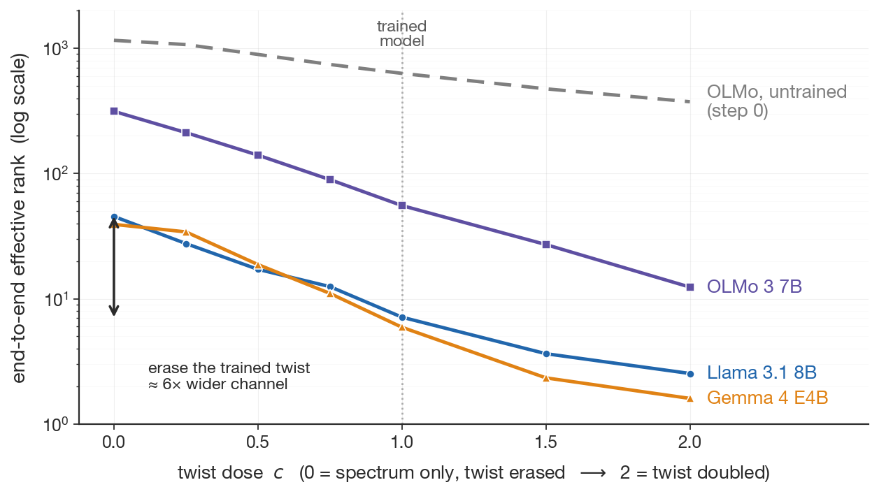
The experiment: take each layer’s Jacobian, decompose it, and put a knob on the non-normal piece. Call the setting c:
At c = 1, we leave the non-normal part exactly as trained. This is the real model.
At c = 0, we erase the non-normal part entirely while keeping every eigenvalue exactly where it was. This is a hypothetical model with the trained spectrum but none of the trained twist—suspect one alone, suspect two surgically removed.
At c = 2, we double the non-normal part, again leaving the spectrum fixed.
Then, at each setting, we recompose the whole stack and remeasure the effective rank of the end-to-end map. If the bottleneck is the eigenvalues’ doing, dialing the non-normal part to zero should change nothing—the spectrum is untouched, so the funnel should hold. If it’s the non-normal structure’s doing, the funnel should open up the moment we turn the knob down.
The funnel opens up. In Llama, turning the knob to zero—keeping every eigenvalue, deleting only the trained twist—lifts the effective rank from about 7 to about 45, a sixfold widening of the channel. The other models do the same thing: OLMo goes from roughly 56 to 314, Gemma from about 6 to 39. And turning the knob past the trained setting, to c = 2, squeezes the channel even tighter—down to about 2.5 in Llama. The bottleneck tracks the non-normal structure up and down, smoothly, like a dose-response curve. The spectrum, by itself, doesn’t produce the funnel. The trained twist does.
Two obvious objections, both of which we headed off. Maybe it’s not the twist’s specific structure—maybe any matrix of that size, added in, would do it. So we replaced the trained non-normal part with a random one of the exact same magnitude. That didn’t reproduce the funnel; it reversed it, pushing the effective rank up into the hundreds. The bottleneck depends on the particular trained structure, not on the mere amount of off-diagonal mass. And maybe it’s an artifact of the residual connection—the “+1” skip that every layer adds to itself. So we redid the entire surgery on the layer’s computation with the skip stripped out. Same dose-response, essentially unchanged. The funnel is a property of what the layers learned to compute, not of the architecture’s bookkeeping.
And the untrained model is the quiet confirmation in the corner of the plot. Run the same knob on OLMo at step 0, and the curve is nearly flat—turning the twist up or down barely moves the effective rank, because at initialization there’s no trained twist to remove. The dose-response is the training signal.
What this buys us
The headline from the last post was that training installs a geometry—rotation early, symmetry late—across the depth of the network. This post adds a second learned object and ties it to the first.
The bottleneck is learned, and we can now say where it lives: not in the eigenvalues of the trained Jacobians, but in their non-normal structure—the same lopsided, input-output-misaligned property that produced the rotations. That’s a more precise claim than “training compresses representations.” It’s a claim about which mathematical feature of the trained operator carries the compression, and it’s hard to make from looking at features or circuits alone. You have to look at the operator, and you have to be able to take it apart.
What we can’t yet say is what survives in those seven directions. They’re clearly load-bearing—they’re the only directions through which the input can still reach the output—so it would be good to know what they encode. Do they have an outsize impact on perplexity? Do they line up with the directions the logit lens reads out? With known feature subspaces? These are clear next questions in this line of work.
It’s also worth saying that we’re not alone at these bottleneck statistics. Other groups, using mathematical objects quite different from ours, keep landing in the same neighborhood: detached Jacobians with the nonlinearities frozen (stable rank around one to three), least-squares linear maps fit between layers (a compression-then-expansion cycle), even vision transformers analyzed by yet another method. Different tools, different architectures, the same shape of answer—computation funnels down through depth into a handful of dimensions. When several methods that share none of each other’s assumptions converge on the same result, the result is probably real.
There’s another thread worth pulling, and it’s the subject of the next post. The residual stream’s coordinates aren’t an undifferentiated soup—they organize into communities, clusters of units that move together. The handful of directions that survive the bottleneck and the community structure of the stream are, we suspect, two views of the same underlying organization. Connecting them is where this series goes next.